import numpy as np
import pandas as pd

df_ads = pd.read_csv('/kaggle/input/advertising-simple-dataset/advertising.csv')
df_ads.head()
Loading...
import matplotlib.pyplot as plt
import seaborn as sns
# 对所有的标签和特征两两显示其相关性的热力图
sns.heatmap(df_ads.corr(), cmap="YlGnBu", annot=True)
plt.show()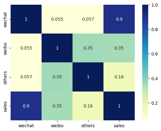
# 显示销售额和各种广告投放金额的散点图
sns.pairplot(df_ads,
            x_vars = ['wechat', 'weibo', 'others'],
            y_vars = 'sales',
            height = 4, aspect = 1, kind = 'scatter')

plt.show()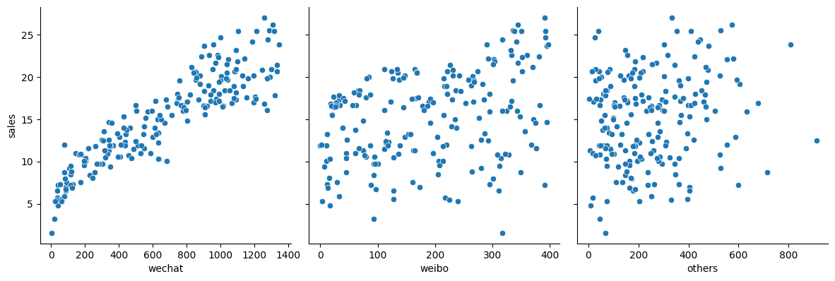
# 构建特征集,只含有微信公众号广告投放金额的一个特征
X = np.array(df_ads.wechat)
# 构建标签集,销售额
y = np.array(df_ads.sales)
print("张量 X 的阶:", X.ndim)
print("张量 X 的形状:", X.shape)
print("张量 X 的内容:", X)
张量 X 的阶: 1
张量 X 的形状: (200,)
张量 X 的内容: [ 304.4 1011.9 1091.1 85.5 1047. 940.9 1277.2 38.2 342.6 347.6
980.1 39.1 39.6 889.1 633.8 527.8 203.4 499.6 633.4 437.7
334. 1132. 841.3 435.4 627.4 599.2 321.2 571.9 758.9 799.4
314. 108.3 339.9 619.7 227.5 347.2 774.4 1003.3 60.1 88.3
1280.4 743.9 805.4 905. 76.9 1088.8 670.2 513.7 1067. 89.2
130.1 113.8 195.7 1000.1 283.5 1245.3 681.1 341.7 743. 976.9
1308.6 953.7 1196.2 488.7 1027.4 830.8 984.6 143.3 1092.5 993.7
1290.4 638.4 355.8 854.5 3.2 615.2 53.2 401.8 1348.6 78.3
1188.9 1206.7 899.1 364.9 854.9 1099.7 909.1 1293.6 311.2 411.3
881.3 1091.5 18.7 921.4 1214.4 1038.8 427.2 116.5 879.1 971.
899.1 114.2 78.3 59.6 748.5 681.6 261.6 1083.8 1322.7 753.5
1259.9 1080.2 33.2 909.1 1092.5 1208.5 766.2 467.3 611.1 202.5
24.6 442.3 1301.3 314.9 634.7 408.1 560.1 503.7 1154.8 1130.2
932.8 958.7 1044.2 1274.9 550.6 1259. 196.1 548.3 650.2 81.4
499.6 1033.8 219.8 971.4 779.4 1019.2 1141.6 994.2 986.4 1318.1
300.8 588.8 1056.1 179.7 1080.2 255.7 1011.9 941.4 928.7 167.9
271.2 822.6 1162.1 596.5 990.5 533.3 1335.9 308.5 1106.6 805.4
1002.4 347.6 443.6 389.9 642.9 243.4 841.3 35.5 85.1 784.9
428.6 173.8 1037.4 712.5 172.9 456.8 396.8 1332.7 546.9 857.2
905.9 475.9 959.1 125.1 689.3 869.5 1195.3 121.9 343.5 796.7]
# 通过 reshape 方法把向量转换为矩阵
X = X.reshape((len(X), 1))
# 通过 reshape 方法把向量转换为矩阵
y = y.reshape((len(y), 1))

print("张量 X 的阶:", X.ndim)
print("张量 X 的形状:", X.shape)
print("张量 X 的内容:", X)
张量 X 的阶: 2
张量 X 的形状: (200, 1)
张量 X 的内容: [[ 304.4]
[1011.9]
[1091.1]
[ 85.5]
[1047. ]
[ 940.9]
[1277.2]
[ 38.2]
[ 342.6]
[ 347.6]
[ 980.1]
[ 39.1]
[ 39.6]
[ 889.1]
[ 633.8]
[ 527.8]
[ 203.4]
[ 499.6]
[ 633.4]
[ 437.7]
[ 334. ]
[1132. ]
[ 841.3]
[ 435.4]
[ 627.4]
[ 599.2]
[ 321.2]
[ 571.9]
[ 758.9]
[ 799.4]
[ 314. ]
[ 108.3]
[ 339.9]
[ 619.7]
[ 227.5]
[ 347.2]
[ 774.4]
[1003.3]
[ 60.1]
[ 88.3]
[1280.4]
[ 743.9]
[ 805.4]
[ 905. ]
[ 76.9]
[1088.8]
[ 670.2]
[ 513.7]
[1067. ]
[ 89.2]
[ 130.1]
[ 113.8]
[ 195.7]
[1000.1]
[ 283.5]
[1245.3]
[ 681.1]
[ 341.7]
[ 743. ]
[ 976.9]
[1308.6]
[ 953.7]
[1196.2]
[ 488.7]
[1027.4]
[ 830.8]
[ 984.6]
[ 143.3]
[1092.5]
[ 993.7]
[1290.4]
[ 638.4]
[ 355.8]
[ 854.5]
[ 3.2]
[ 615.2]
[ 53.2]
[ 401.8]
[1348.6]
[ 78.3]
[1188.9]
[1206.7]
[ 899.1]
[ 364.9]
[ 854.9]
[1099.7]
[ 909.1]
[1293.6]
[ 311.2]
[ 411.3]
[ 881.3]
[1091.5]
[ 18.7]
[ 921.4]
[1214.4]
[1038.8]
[ 427.2]
[ 116.5]
[ 879.1]
[ 971. ]
[ 899.1]
[ 114.2]
[ 78.3]
[ 59.6]
[ 748.5]
[ 681.6]
[ 261.6]
[1083.8]
[1322.7]
[ 753.5]
[1259.9]
[1080.2]
[ 33.2]
[ 909.1]
[1092.5]
[1208.5]
[ 766.2]
[ 467.3]
[ 611.1]
[ 202.5]
[ 24.6]
[ 442.3]
[1301.3]
[ 314.9]
[ 634.7]
[ 408.1]
[ 560.1]
[ 503.7]
[1154.8]
[1130.2]
[ 932.8]
[ 958.7]
[1044.2]
[1274.9]
[ 550.6]
[1259. ]
[ 196.1]
[ 548.3]
[ 650.2]
[ 81.4]
[ 499.6]
[1033.8]
[ 219.8]
[ 971.4]
[ 779.4]
[1019.2]
[1141.6]
[ 994.2]
[ 986.4]
[1318.1]
[ 300.8]
[ 588.8]
[1056.1]
[ 179.7]
[1080.2]
[ 255.7]
[1011.9]
[ 941.4]
[ 928.7]
[ 167.9]
[ 271.2]
[ 822.6]
[1162.1]
[ 596.5]
[ 990.5]
[ 533.3]
[1335.9]
[ 308.5]
[1106.6]
[ 805.4]
[1002.4]
[ 347.6]
[ 443.6]
[ 389.9]
[ 642.9]
[ 243.4]
[ 841.3]
[ 35.5]
[ 85.1]
[ 784.9]
[ 428.6]
[ 173.8]
[1037.4]
[ 712.5]
[ 172.9]
[ 456.8]
[ 396.8]
[1332.7]
[ 546.9]
[ 857.2]
[ 905.9]
[ 475.9]
[ 959.1]
[ 125.1]
[ 689.3]
[ 869.5]
[1195.3]
[ 121.9]
[ 343.5]
[ 796.7]]
# 将数据集进行80%(训练集)和20%(测试集)的分割
from sklearn.model_selection import train_test_split
X_train, X_test, y_train, y_test = train_test_split(X, y, test_size = 0.2, random_state = 0)
# 定义归一化函数,进行数据压缩
def scaler(train, test):
min = train.min(axis = 0)
max = train.max(axis = 0)
gap = max - min
train -= min
train /= gap
test -= min
test /= gap
return train, test
# 对特征归一化
X_train, X_test = scaler(X_train, X_test)
# 对标签也归一化
y_train, y_test = scaler(y_train, y_test)
# 用之前已经导入的matplotlib.pyplot中的 plot 方法显示散点图
plt.plot(X_train, y_train, 'r.', label = 'Training data')
plt.xlabel('wechat')
plt.ylabel('sales')
plt.legend()
plt.show()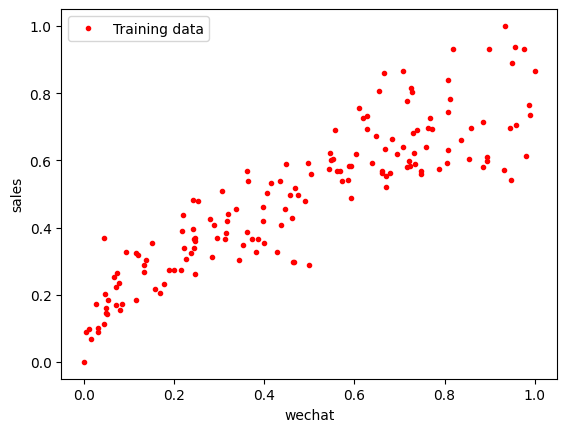
def loss_function(X, y, weight, bias):
    y_hat = weight * X + bias
    loss = y_hat - y
    cost = np.sum(loss**2)/(2*len(X))

    return cost

print("当权重为 5,偏置为 3 时,损失为:",
    loss_function(X_train, y_train, weight = 5, bias = 3))
print("当权重为 100,偏置为 1 时,损失为:",
    loss_function(X_train, y_train, weight = 100, bias = 1))
当权重为 5,偏置为 3 时,损失为: 12.79639097078006
当权重为 100,偏置为 1 时,损失为: 1577.9592615030556
def gradient_decent(X, y, w, b, lr, iter):
    # 初始化记录梯度下降过程中损失的数组
    l_history = np.zeros(iter)
    # 初始化记录梯度下降过程中权重的数组
    w_history = np.zeros(iter)
    # 初始化记录梯度下降过程中偏置的数组
    b_history = np.zeros(iter)

    # 进行梯度下降的迭代,就是下多少级台阶
    for i in range(iter):
        y_hat = w * X + b
        loss = y_hat - y
        # 对权重求导
        derivative_weight = X.T.dot(loss) / len(X)
        # 对偏置求导
        derivative_bias = sum(loss) * 1/len(X)
        # 结合学习速率更新权重
        w = w - lr * derivative_weight
        # 结合学习速率更新偏置
        b = b - lr * derivative_bias
        # 梯度下降过程中损失的历史记录
        l_history[i] = loss_function(X, y, w, b)
        # 梯度下降过程中权重的历史记录
        w_history[i] = w
        # 梯度下降过程中偏置的历史记录
        b_history[i] = b

    return l_history, w_history, b_history

iterations = 100
alpha = 1
weight = -5
bias = 3

print('当前损失:', loss_function(X_train, y_train, weight, bias))
当前损失: 1.343795534906634
plt.plot(X_train, y_train, 'r.', label = 'Training data')
# X 值域
line_X = np.linspace(X_train.min(), X_train.max(), 500)
line_y = [weight * x + bias for x in line_X]
plt.plot(line_X, line_y, 'b--', label = 'Current hypothesis')
plt.xlabel('wechat')
plt.ylabel('sales')
plt.legend()
plt.show()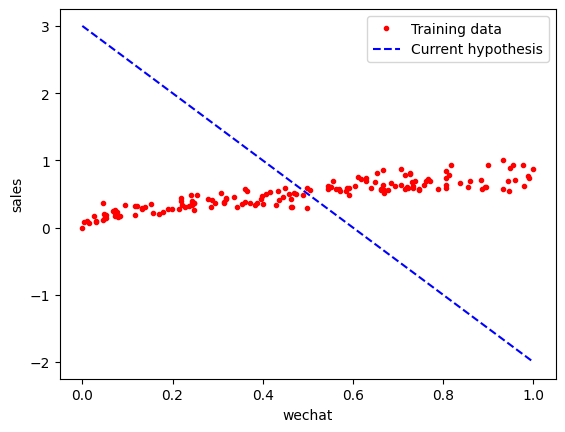
loss_history, weight_history, bias_history = gradient_decent(
    X_train, y_train, weight, bias, alpha, iterations
)
<ipython-input-9-02fa0a77783a>:24: DeprecationWarning: Conversion of an array with ndim > 0 to a scalar is deprecated, and will error in future. Ensure you extract a single element from your array before performing this operation. (Deprecated NumPy 1.25.)
w_history[i] = w
<ipython-input-9-02fa0a77783a>:26: DeprecationWarning: Conversion of an array with ndim > 0 to a scalar is deprecated, and will error in future. Ensure you extract a single element from your array before performing this operation. (Deprecated NumPy 1.25.)
b_history[i] = b
plt.plot(loss_history, 'g--', label = 'Loss Curve')
plt.xlabel('Iterations')
plt.ylabel('Loss')
plt.legend()
plt.show()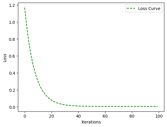
plt.plot(X_train, y_train, 'r.', label = 'Training data')
line_X = np.linspace(X_train.min(), X_train.max(), 500)
line_y = [weight_history[-1] * x + bias_history[-1] for x in line_X]
plt.plot(line_X, line_y, 'b--', label='Current hypothesis')
plt.xlabel('wechat')
plt.ylabel('sales')
plt.legend()
plt.show()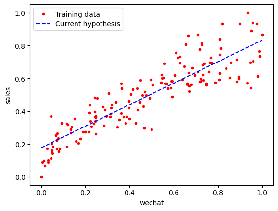
print('测试集损失:', loss_function(X_test, y_test, weight_history[-1], bias_history[-1]))测试集损失: 0.00458180938024721